🏦 Loan Default Prediction Challenge
How I developed a machine learning model that could accurately predict who would default on their loan

I recently took part in the Load Default Prediction Challenge on Zindi. In this blog post, I’m going to provide you with a detailed description of the analysis I conducted, together with the final recommendations I provided with regards to the types of customers who are more and less likely to default on their loans.
1. The problem
SuperLender is a local digital lending company who prides themselves in delivering profitable and high-impact loan alternatives to the people of Nigeria. The company has approached the Zindi community to develop an effective credit risk model to predict the odds that a returning customer will repay their loan. More specifically, they recommended that the approach should be based on two main risk drivers of loan default prediction: (1) The willingness and (2) the ability of a customer to pay back their loan.
2. The data
SuperLender provided us with three separate sets of data namely: (1) Performance data, (2) previous loans data and (3) demographic data. A breakdown of the features, data types and descriptions for the performance, previous loans and demographics datasets are provided in Tables 1, 2 and 3, respectively. The performance dataset contains repeat loans taken by customers and contains a binary feature good_bad_flag indicating whether the customer settled their loan on time or not — this feature serves at the target variable. The previous loans dataset contains all previous loans that a customer in the performance dataset took out prior to the loan. And finally, the demographics dataset contains demographic information corresponding to each customer in the performance dataset. All three of the aforementioned datasets are related via the customer_id key.
| # | Feature name | Data type | Description |
|---|---|---|---|
| 1 | customer_id | Meta | Primary key |
| 2 | system_loan_id | Meta | The ID associated with the particular loan |
| 3 | loan_number | Continuous | The number of the loan |
| 4 | approved_date | Timestamp | Date that loan was approved |
| 5 | creation_date | Timestamp | Date that loan application was created |
| 6 | loan_amount | Continuous | Loan value taken |
| 7 | total_due | Continuous | Total repayment required to settle the loan |
| 8 | term_days | Continuous | Term of loan |
| 9 | referred_by | Meta | The customer_id of the referral customer |
| 10 | good_bad_flag | Categorical | Whether the customer settled their loan on time or not |
| # | Feature name | Data type | Description |
|---|---|---|---|
| 1 | customer_id | Meta | Primary key |
| 2 | system_loan_id | Meta | The ID associated with the particular loan |
| 3 | loan_number | Continuous | The number of the loan |
| 4 | approved_date | Timestamp | Date that loan was approved |
| 5 | creation_date | Timestamp | Date that loan application was created |
| 6 | loan_amount | Continuous | Loan value taken |
| 7 | total_due | Continuous | Total repayment required to settle the loan |
| 8 | closed_date | Timestamp | Date that the loan was settled |
| 9 | referred_by | Meta | The customer_id of the referral customer |
| 10 | first_due_date | Timestamp | Date of first payment due |
| 11 | first_repaid_date | Timestamp | Actual date that customer paid the first payment |
| # | Feature name | Data type | Description |
|---|---|---|---|
| 1 | customer_id | Meta | Primary key |
| 2 | birth_date | Timestamp | Date of birth of the customer |
| 3 | bank_account_type | Categorical | Type of primary bank account |
| 4 | longitude_gps | Continuous | Longitude of customer |
| 5 | latitude_gps | Continuous | Latitude of customer |
| 6 | bank_name_clients | Categorical | Name of customer's bank |
| 7 | bank_branch_clients | Categorical | Location of customer's branch |
| 8 | employment_status_clients | Categorical | Customer's type of employment |
| 9 | level_of_education_clients | Categorical | Customer's highest level of education |
3. Methodology
This section contains a description of the methodology followed during this investigation. The section opens in §3.1 with a description of the features constructed in order to draw more information from the three sets of data. This is followed, in §3.2, by an elucidation of the data mining architecture constructed for the purpose of this analysis.
3.1. Feature engineering
Arguably, the most involved and important tasks in the data mining process is that of feature engineering which requires the data scientist to construct informative features based on one or more feature(s) currently present in the data
In the previous loans dataset, the number of days a customer’s loan was over/under the days stipulated by the loan’s term is defined mathematically as
\begin{equation} \mbox{days_over_under}=\mbox{close_date}-(\mbox{approve_date}+\mbox{term_days}).\label{daysoverunder} \end{equation}
The expression in (\ref{daysoverunder}) is used as a basis to construct the first new feature default_loan in the previous loans dataset indicating whether the customer had defaulted on their loan, defined mathematically as
\begin{equation} \mbox{default_loan}=0\mbox{ if days_over_under}\leq 0\mbox{ otherwise }1.\label{3.eqn.defaultloan} \end{equation}
The expression in (\ref{3.eqn.defaultloan}) is also used to construct a second feature days_over in the previous loans dataset indicating the number of days a customer took to pay the loan after the agreed term days, defined mathematically as
\begin{equation} \mbox{days_over}=\mbox{default_loan}\times\mbox{days_over_under},\label{3.eqn.daysover} \end{equation}
In the performance dataset, the result computed in (\ref{3.eqn.defaultloan}) is then used to construct a new feature prev_default_loan $={\tt SUM}($ default_loan $)$ in the performance dataset indicating the total number of loans a customer has previously defaulted on. The result computed in (\ref{3.eqn.daysover}) is then used to construct a new feature prev_days_over $={\tt SUM}($ days_over $)$ in the performance dataset indicating the total days a customer has exceeded their payment terms on past loans. A feature prop_default_loan is also constructed in the performance dataset indicating the proportion of loans a customer has previously defaulted on, defined mathematically as
\begin{equation} \mbox{prop_default_loan}=\frac{\mbox{prev_default_loan}}{\mbox{loan_number}-1},\label{3.eqn.propdefaultloan} \end{equation}
where prev_default_loan $={\tt SUM}($ default_loan $)$ is a new feature indicating the total number of loans a customer has previously defaulted on and $\mbox{loan_number}$ is the loan number of the current loan. The interest rate charged to each customer is defined mathematically as
\begin{equation} \mbox{interest_per_day}=\frac{\mbox{total_due}-\mbox{loan_amount}}{\mbox{term_days}}.\label{3.eqn.interestperday} \end{equation}
The result computed in (\ref{3.eqn.interestperday}) is used as a basis to construct a new feature prop_interest_per_day in the performance loans dataset indicating the proportion of customer’s interest rate on their current and previous loans, defined mathematically as
\begin{equation} \mbox{prop_interest_per_day}=\frac{\mbox{interest_per_day}-\mbox{prev_interest_per_day}}{\mbox{prev_interest_per_day}},\label{3.eqn.propinterestperday} \end{equation}
where prev_interest_per_day $={\tt AVG}($ interest_per_day $)$ is a new feature indicating the average interest rate charged to a customer on their previous loans. In the same way, a new feature prop_term_days is constructed in the performance dataset indicating the proportion of customer’s loan terms on their current and previous loans, defined mathematically as
\begin{equation} \mbox{prop_term_days}=\frac{\mbox{term_days}-\mbox{prev_term_days}}{\mbox{prev_term_days}},\label{3.eqn.proptermdays} \end{equation}
where prev_term_days $={\tt AVG}($ term_days $)$ is a new feature indicating the average term days offered to the customer on their previous loans. And finally, a new feature prop_loan_amount is constructed to indicate the proportion of customer’s loan amount on their current and previous loans, defined mathematically as
\begin{equation} \mbox{prop_loan_amount}=\frac{\mbox{loan_amount}-\mbox{prev_loan_amount}}{\mbox{prev_loan_amount}},\label{3.eqn.proploanamount} \end{equation}
where prev_loan_amount$={\tt AVG}($ loan_amount $)$ is a new feature indicating a customer’s average previous loan amounts.
In the demographics dataset, a new feature age is constructed indicating the age of the customer in years, defined mathematically as
\begin{equation} \mbox{age}=\mbox{now}-\mbox{birthdate},\label{3.eqn.age} \end{equation}
where now indicates the current time in years.
3.2. Data mining architecture
A data mining solution was built in the Orange Data Mining Software interest_per_day feature is then computed according to expression (\ref{3.eqn.interestperday}) using Widget A3 and are passed to Widget A4. The term_days, loan_number, loan_amount and interest_per_day, good_bad_flag and customer_id features are then selected in Widget A4 and are passed to Widget C1.
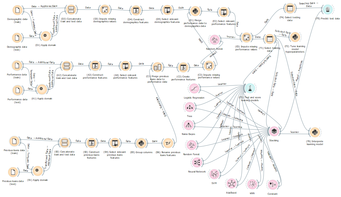
Given the training and testing previous loans data, these datasets are first formatted and concatenated into a single dataset using Widgets B1 and B2, respectively, and are passed to Widget B3. The default_loan, days_over and interest_per_day features are then computed according to expressions (\ref{3.eqn.defaultloan}), (\ref{3.eqn.daysover}) and (\ref{3.eqn.interestperday}), respectively, using Widget B3 and are passed to Widget B4. The days_over, default_loan, loan_amount and term_days, interest_per_day and customer_id features are then selected in Widget B4 and passed to Widget B5. Widget B5 is a Python script used to group the multiple previous loan records associated with each customer_id into a single representative record which are then passed to Widget B6. In this script, the days_over and defaulted_loan features are summed, while the loan_amount, term_days and interest_per_day features are averaged. In Widget B6, the days_over, defaulted_loan, loan_amount, term_days and interest_per_day features are renamed to prev_days_over, prev_defaulted_loan, prev_loan_amount, prev_term_days and prev_interest_per_day, respectively, and are passed to Widget C1.
The previous loans data is now merged to the performance data using Widget C1 and are passed to Widget C2. The prop_default_loan, prop_interest_per_day, prop_term_days and prop_loan_amount features are then computed according to expressions (\ref{3.eqn.propdefaultloan}), (\ref{3.eqn.propinterestperday}), (\ref{3.eqn.proptermdays}) and (\ref{3.eqn.proploanamount}), respectively, using Widget C2 and are passed to Widget C3. As this stage, any missing values are filled in using Widget C3 by employing a model-based imputing strategy, where a Random Forest (RF) learning model is used predict the values of missing data points based on the values of a corresponding record.
Given the training and testing demographics data, these datasets are first formatted and concatenated into a single dataset using Widgets D1 and D2, respectively, and are passed to Widget D3. In Widget D3, the employment_status_clients and level_of_education_clients are imputed based on the highest category frequency and are passed to Widget D4. The age feature is then computed according to expression (\ref{3.eqn.age}) using Widget D4 and are passed to Widget D5. The age, bank_account_type, bank_name_clients, employment_status_clients and level_of_eduction_clients and customer_id features are then selected in Widget D5 and are passed to Widget E1.
Widget E1 is a Python script used to merge the demographics data to the performance data which is then passed to Widget E2. The term_days, loan_amount, interest_per_day, prev_days_over, prop_default_loan, prop_interest_per_day, prop_term_days, prop_loan_amount, age, bank_account_type, bank_name_clients, employment_status_clients and level_of_eduction_clients and customer_id features features are then selected in Widget E2 and are passed to Widget E3. Any missing values are again filled in using Widget E3 via a RF model-based imputation method.
The dataset is then partitioned into the training and testing dataset in Widgets F1 and F4, respectively. A set of learning models are then tested and scored in Widget F3 by employing a $k$-fold cross validation splitting criterion. The best learning model is then used in Widget F4 to predict the classes of the testing dataset. Widget F6 may finally be employed to produce a rule formulation for a specified learning model.
4. Data exploration
This section is dedicated to exploring the data used and produced by the data mining architecture described in §3.2. Data distribution, spatial and temporal analyses are conducted in §4.1, §4.2 and §4.3, respectively, in order to draw some preliminary insights from the data supplied from SuperLender which may better guide the predictive modelling component of this investigation.
4.1. Data distribution analysis
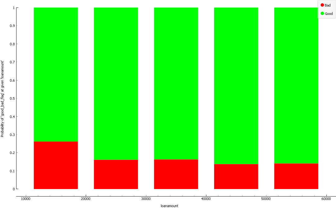
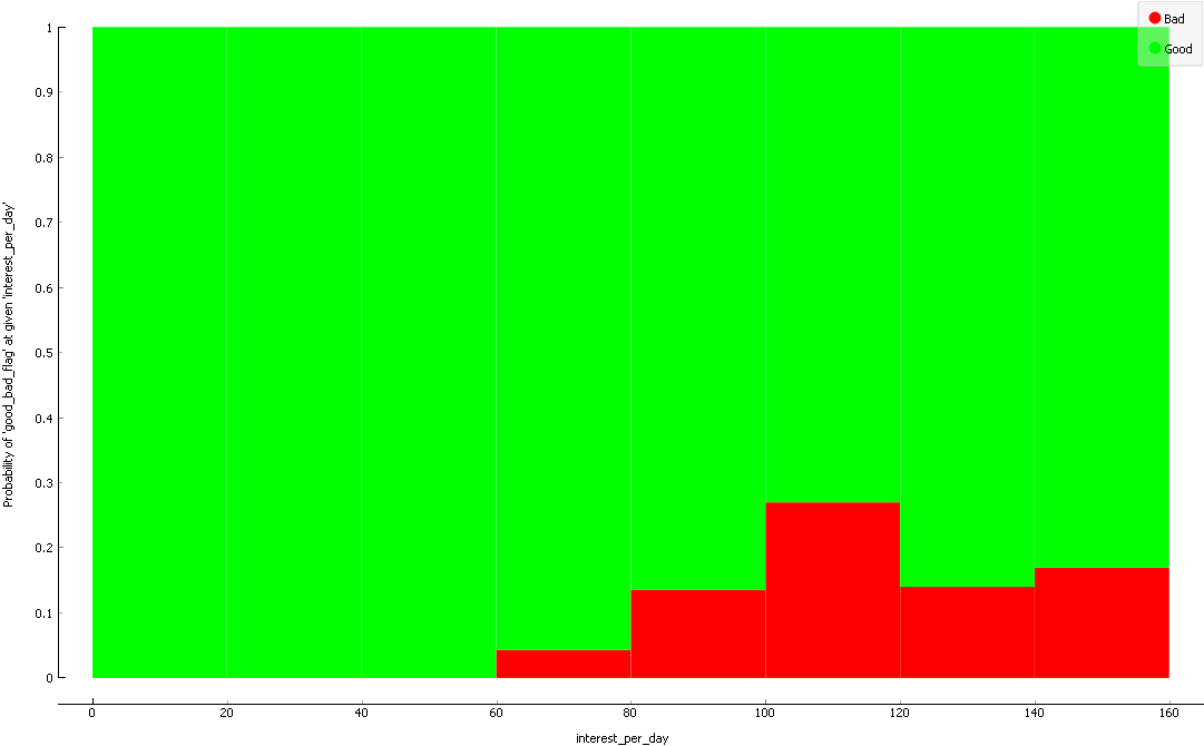
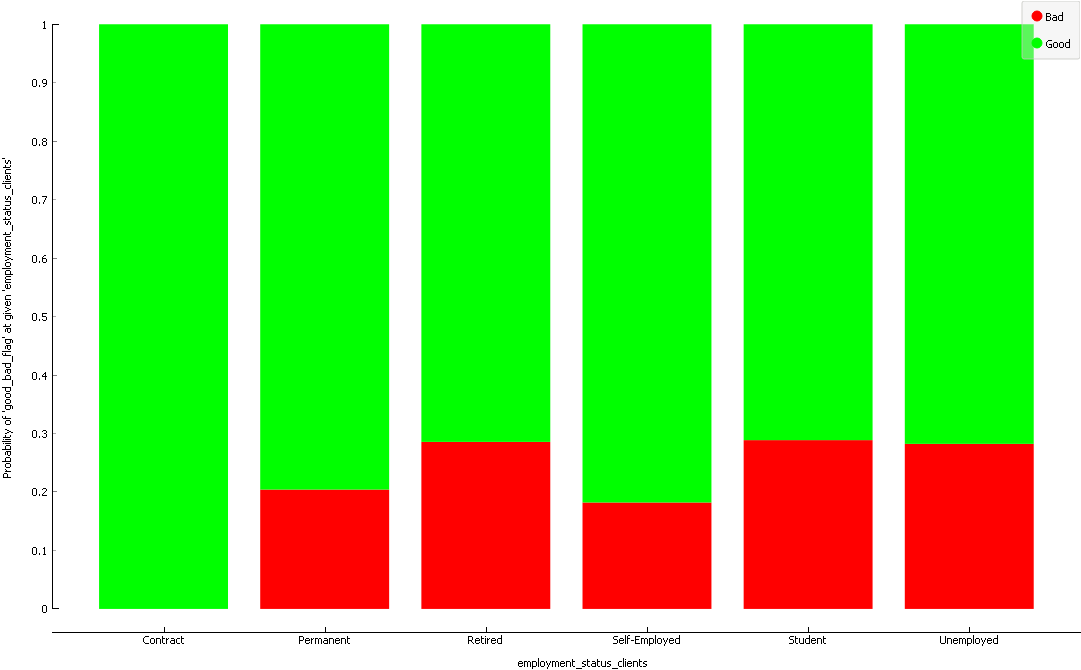
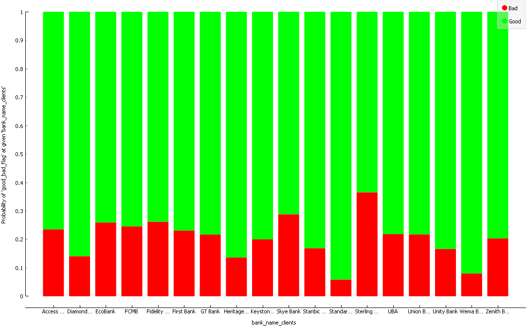
As may be seen in Figure 2(a), a higher proportion of customers who take out smaller loans (less than $20\,000$ Nigerian naira) end up defaulting on their loan. A higher proportion of customers who are charged higher rates of interest per day are also more likely to default on their loan, as illustrated in Figure 2(b). It is also interesting to note that a higher proportion of retired, student and unemployed customers default on their loans, as may be seen in Figur 2(c). And finally, a low proportion of customers banking with Standard Bank and Wema Bank default on their loans while the opposite is true for customers banking with Sterling Bank or Skye Bank.
Moreover, the target variable contains a significantly less customers that have defaulted on their loans than those who have paid their loans. Due to this significantly disproportionate representation among target variable classes, the Area Under the Curve (AUC) (more specifically, the Receiver Operating Characteristic (ROC)) should be employed as an appropriate predictive modelling metric since it is robust against class imbalances.
4.2. Spatial analysis
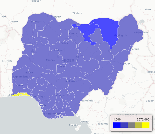
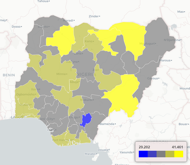
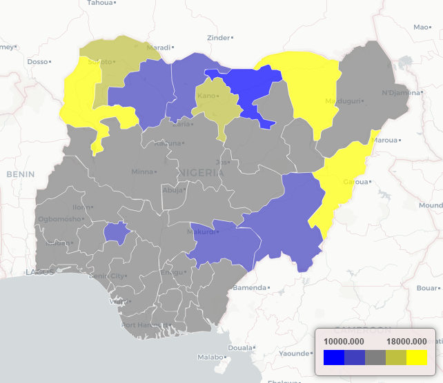
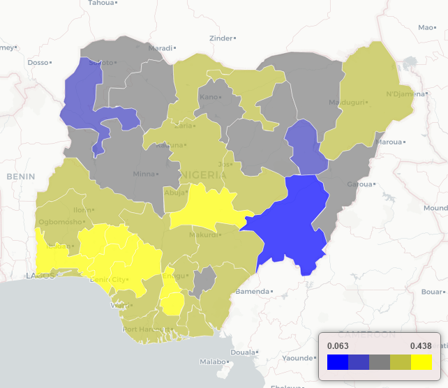
The highest concentration of SuperLender customers are located in the state of Lagos, as may be seen in Figure 3(a), while older customers are typically located in the Zamfara, Jigawa, Yobe and Taraba states, as illustrated in Figure 3(b). As may be seen in Figure 3(c), the highest average loan amounts are observed from customers living in the Kebbi, Yobe and Adamawa states while the largest proportion of customers who default on their loans are located in the Ogun, Lagos, Osun, Ekiti, Ondo, Edo and Nassarawa states, as illustrated in Figure 3(d).
4.3. Temporal analysis
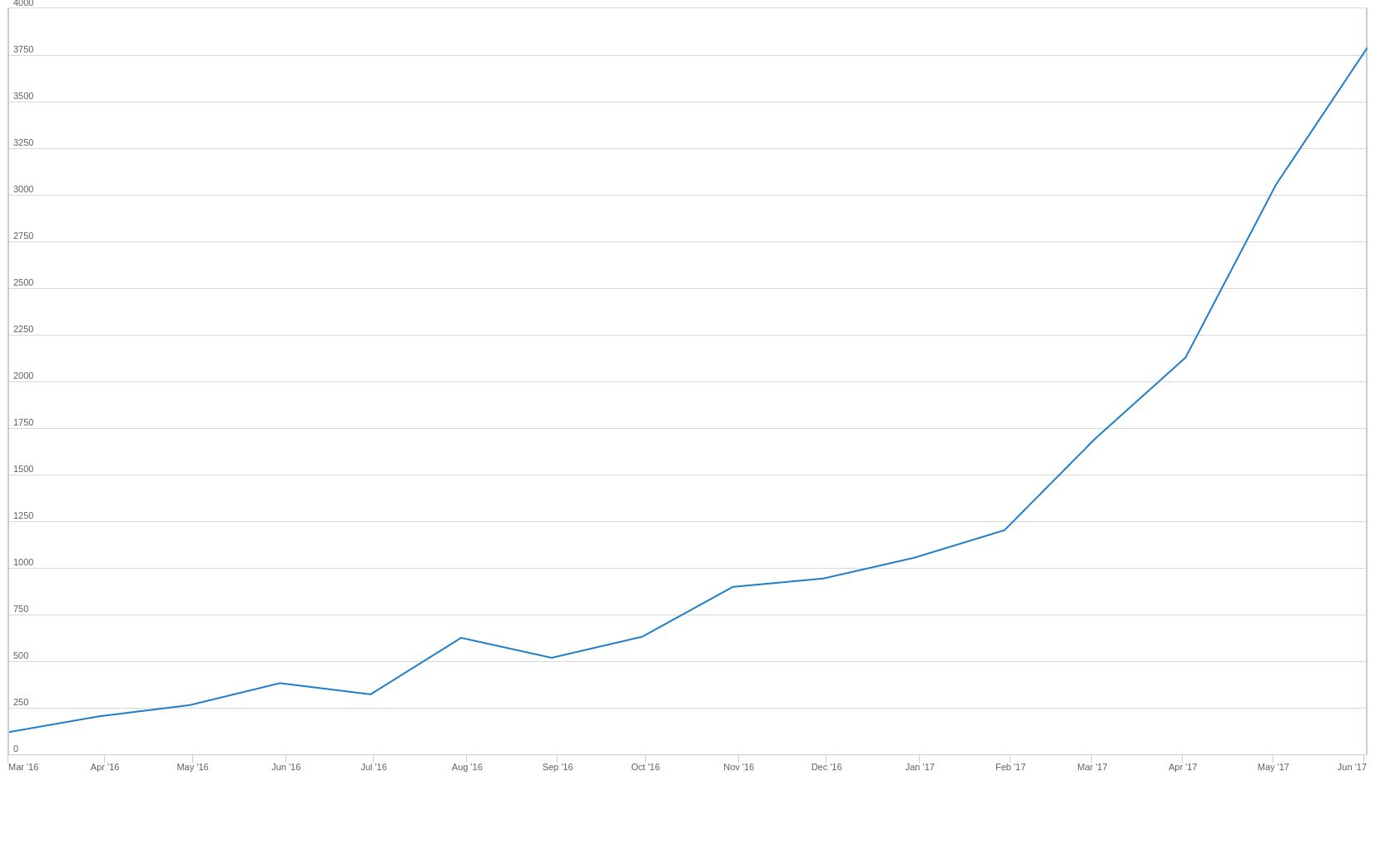
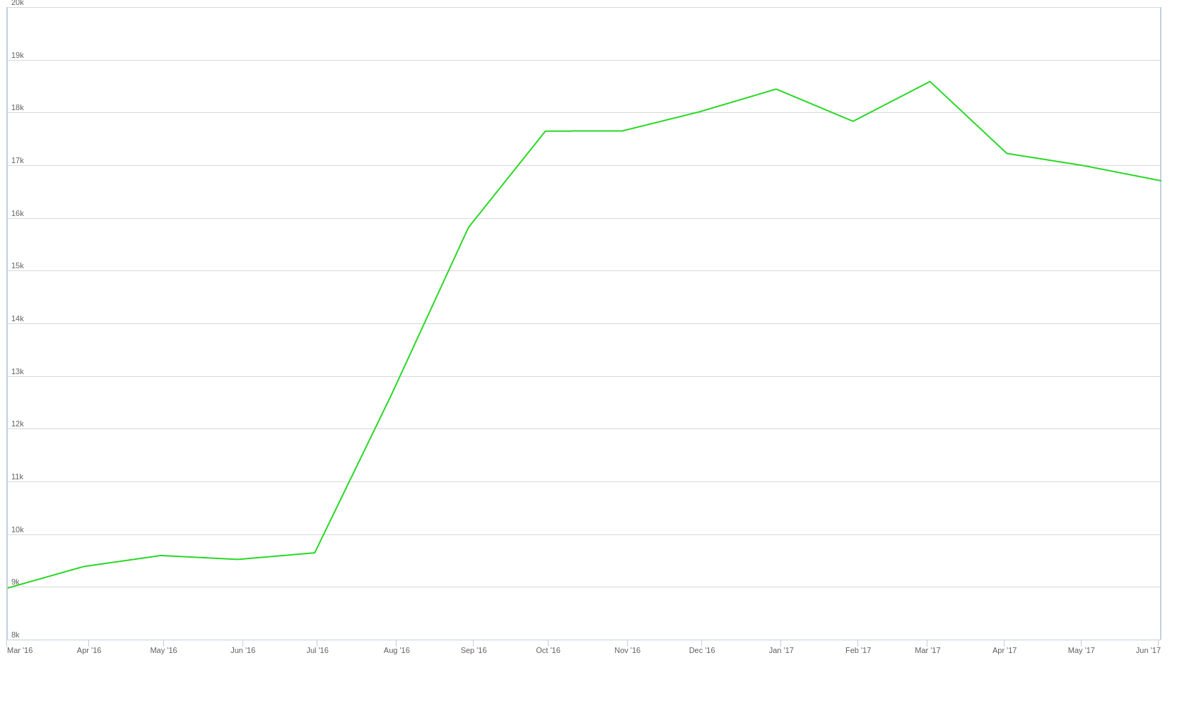
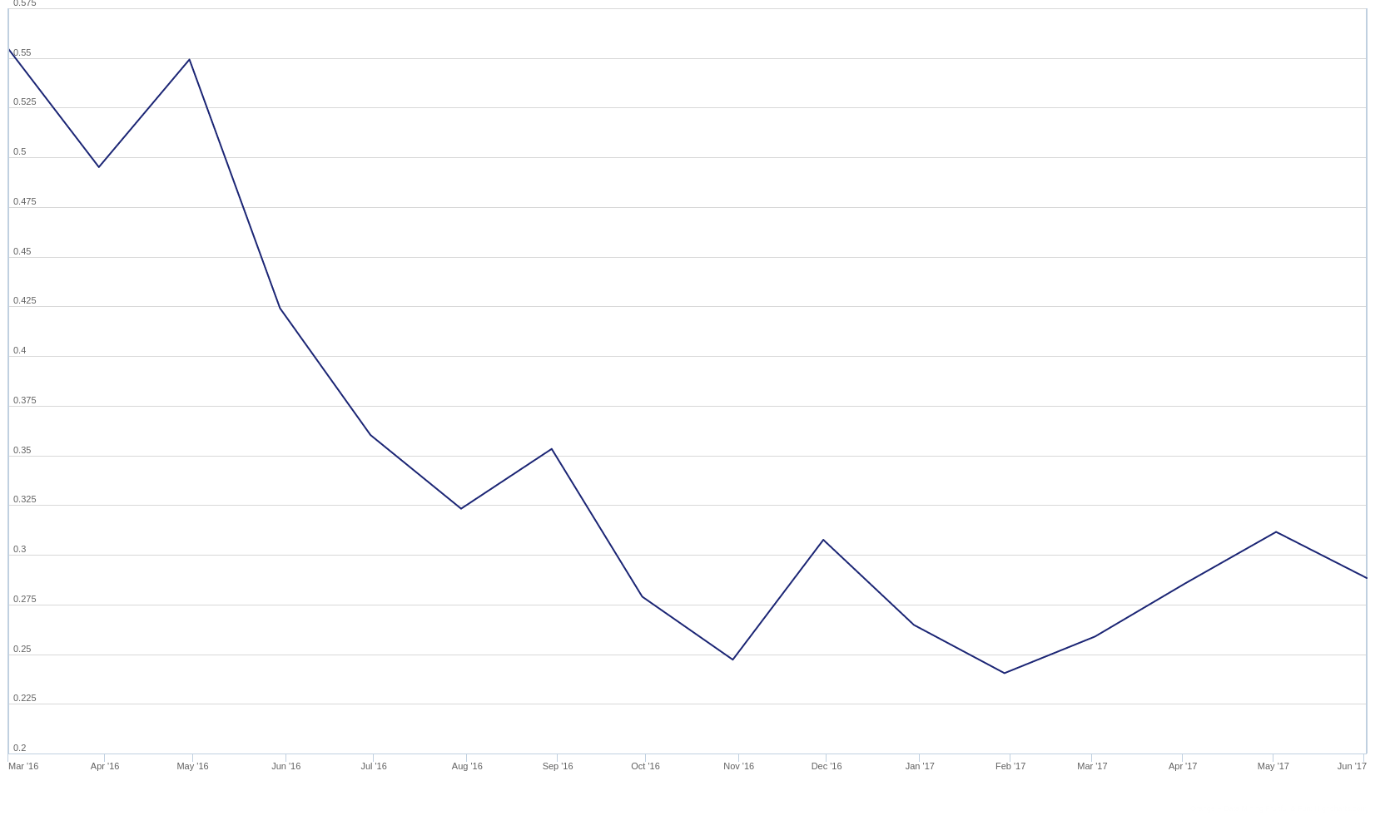
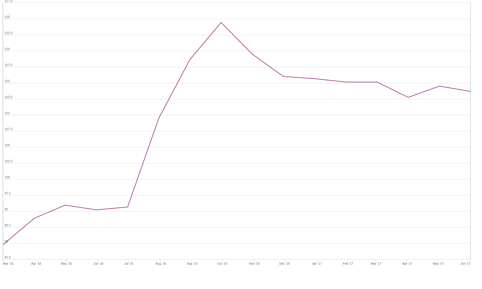
As may be seen in Figure 4(a), the total number of loans issued by SuperLender has drastically increased over the years. Moreover, the average number of customers defaulting on their loans has steadily decreased since May 2016, as illustrated in Figure 4(b). It is also interesting to note that the average amount that SuperLender lends, as shown in Figure 4(c), drastically increased in August 2016. This was accompanied by a sudden increase in the average interest charged on their loans, as may be seen in Figure 4(d). These observations suggest that SuperLender has improved their operations considerably since the end of 2016 and are continuing to grow as a digital lending company in Nigeria.
5. Predictive model results
The purpose of this section is to describe the predictive modelling analysis conducted in this investigation. A description of the hyperparameter tuning procedure is first described in §5.1. This is followed, in §5.2, with a discussion of the predictive capabilities of the selected learning models. And finally, in §5.3, selected learning models are used to identify the most informative features for predicting whether a customer will default on their loan.
5.1. Hyperparameter tuning
A total of eight classification learning models were selected for this predictive investigation, namely the Logistic Regression (LR), Naive Bayes (NB), Classification Tree (CT), RF, k-Nearest Neighbours (kNN), AdaBoost, Support Vector Machine (SVM) and Multi-layer Perceptron (MLP) learning models. Attention then turned to (approximately) optimally tuning the hyper-parameters of each of the learning models by employing a grid-based search technique. The parameters considered in this investigation, together with the (approximately) optimal parameters found in the case of each learning model considered, are as follows:
- LR. In the case of the LR learning model, the L1 and L2 regularisation parameters were considered, together with the regularisation penalty. The best LR learning model employed L1 regularisation and had a regularisation penalty of $12$.
- CT. In the case of the CT learning model, the gini and entropy splitting criteria were considered and the depth of the tree was controlled by imposing a minimum sample number in each leaf. The best CT learning model employed the gini splitting criterion with a minimum of $131$ samples per leaf.
- RF. In the case of the RF learning model, the number of classification trees and the maximum feature subset considered when growing an individual tree were chosen as the appropriate set of parameters. The best RF learning mode employed $190$ classification trees, each considering two random features when growing the tree.
- kNN. In the case of the kNN learning model, the Euclidean, Manhattan and Chebyshev measures were considered as possible distance metrics weighted either uniformly or inversely by distance, together with the number of neighbours parameter. The best kNN learning model considered the ten nearest neighbours based on an uniformly weighted Manhattan distance.
- SVM. In the case of the SVM learning model, a linear, polynomial, sigmoid and radial base function (RBF) kernels where considered, together with the cost penalty term value. The best SVM learning model employed an RBF kernel with a cost penalty term of $1.0$.
- MLP. In the case of the MLP learning model, only network structures with at most two hidden layers and a maximum of thirty neurons (i.e. twice the number of input features) per hidden layer were considered. The ReLu activation function was employed in the case of each MLP structure and optimised the weights of the network according to the Adam optimisation approach. The best structure had two hidden layers, containing $13$ neurons in each layer.
5.2. Model performances
After (approximately) optimal parameter settings had been determined, each learning model was evaluated according to the AUC, Classification Accuracy (CA), F1-score, precision and recall performance metrics in respect of the training set using the 10-fold cross validation splitting criterion. These results may be seen in Table 4 while the ROC for each learning model may be visualised in Figure 5. The well-known stacking method was also used to ensamble all the learning models into a single classifier, where a LR model was employed as an appropriate aggregation model. A constant model which always predicts the target variable mode was also included to serve as a benchmark.
| Model | AUC | CA | F1 | Precision | Recall |
|---|---|---|---|---|---|
| Stack | 0.699 | 0.786 | 0.731 | 0.742 | 0.786 |
| LR | 0.687 | 0.782 | 0.718 | 0.728 | 0.782 |
| CT | 0.681 | 0.778 | 0.716 | 0.718 | 0.778 |
| RF | 0.669 | 0.783 | 0.738 | 0.739 | 0.783 |
| NB | 0.666 | 0.742 | 0.743 | 0.745 | 0.742 |
| MLP | 0.663 | 0.770 | 0.729 | 0.721 | 0.770 |
| SVM | 0.619 | 0.781 | 0.687 | 0.660 | 0.781 |
| AdaBoost | 0.554 | 0.696 | 0.696 | 0.696 | 0.696 |
| kNN | 0.534 | 0.745 | 0.687 | 0.656 | 0.745 |
| Constant | 0.500 | 0.782 | 0.687 | 0.612 | 0.782 |
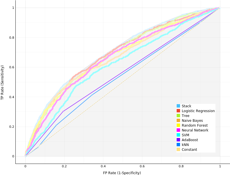
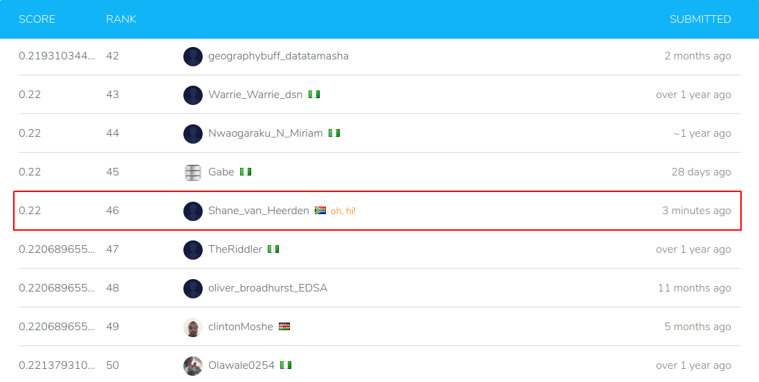
As may be seen from the table, the best performing individual learning model was the LR model achieving an AUC performance of $0.687$, followed closely by the CT model with an AUC of $0.681$. The kNN was the performing learning model achieving an AUC of only $0.534$. The stack learning model ensamble managed to outperform each individual learning model, as expected. This learning model was then used to predict the testing set target variable. These predicted test results were then submitted to the Zindi Data Science Nigeria Challenge
5.3. Model interpretations
Due to the inherent algorithmic structure, learning models can either be white-box or black-box in nature. In a white-box learning model, one can clearly follow the logical rules produced by the model when classifying a specified instance. The rule formulation of a black-box learning model, on the other hand, cannot be interpreted meaningfully by humans. The rule formulation of the LR learning model (a white-box learning model) may, for example, be represented in the form of a nomogram, as illustrated in Figure 7. A nomogram is a diagram that visually represents the rule formulation of selected classifiers by offering an insight into how the values of multiple attributes impact the overall target class probabilities. This is achieved by representing each attribute as a scale, where each point on this scale represents a single value assumed by a feature and the length of a scale signifies the importance of these feature values when describing the value of the target attribute. Features are ranked in descending order on the left-hand axis according to a feature’s absolute importance (i.e. the length of its scale) and the individual dashes (i.e. points) on each explanatory feature scale signifies the importance of the corresponding feature categories when predicting the value bad of the good_bad_flag target variable. In other words, according to the LR model, a dash that lies at the right-most end of a scale signifies an feature value that is the most telling of a customer that defaults on their loan. The inverse is also true: A dash that lies at the left-most end of a scale signifies a feature value which is the most telling of a customer who does not default on their loan. The inverse is also true: A dash that lies at the left-most end of a scale signifies a feature value which is the most telling of a customer who does not default on their loan.
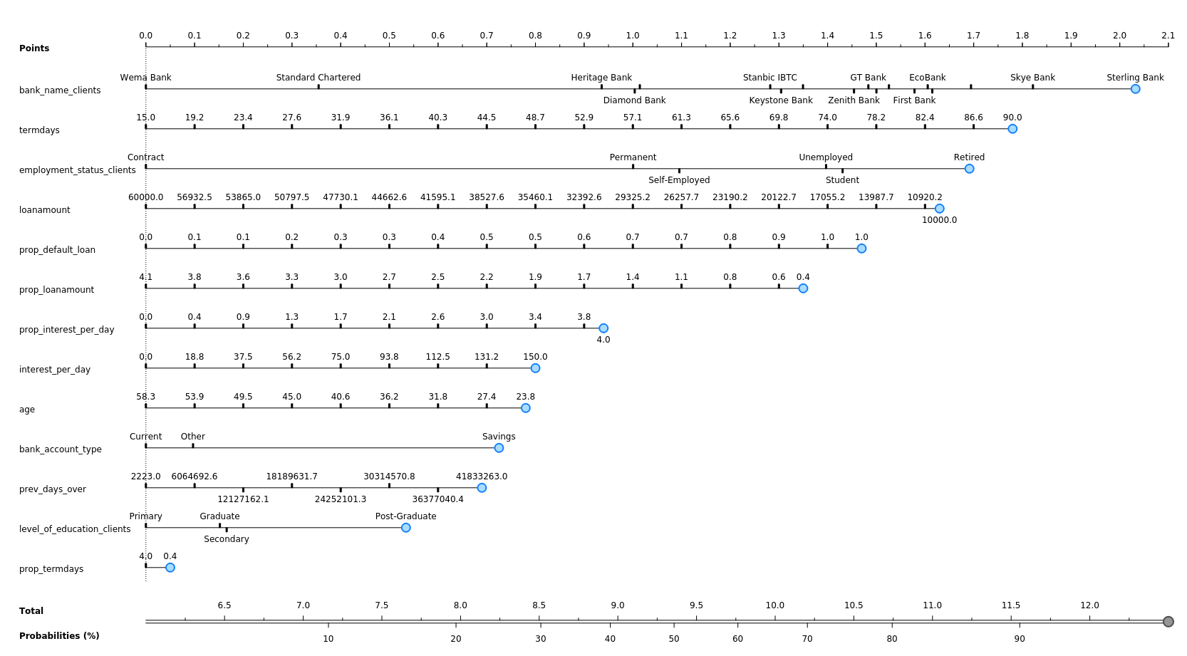
From Figure 7, one may conclude that the most informative feature for the LR learning model was bank_name_clients, where customers who bank with Sterling Bank or Skye Bank are identified as the most likely to default on their current loan. This observation is in agreement with the distribution results observed in Figure 2(d). The second most informative feature is term_days, which suggests that customers who take out a longer loan term are more likely to default on their current loan. The third most informative feature is employment_status_clients which suggests that Retired customers are more likely to default on their current loan. The fourth most informative feature is loan_amount, which suggests that customers who take out smaller loan amounts are more likely to default on their current loan. The fifth most informative feature is prop_default_loan and suggests that customers who have defaulted on a higher proportion of their previous loans are more likely to default on their current loan.
The rule formulation of the CT learning may be seen in the form of a decision tree in Figure 8. As may be seen in the figure, the CT selected to branch first on the prop_default_loan feature and suggests that customers who have previously defaulted on a larger proportion of their loans are more likely to default on their current loan. The second right-most CT branch then selected to branch on the loan_amount feature and suggests that customers who take out loans less than or equal to $10\,000$ Nigerian naira.

6. Conclusion
In this final concluding section, sensible recommendations are provided to SuperLender in §6.1 based on the investigations conducted in this report. The focus then shifts in §6.2 to a discussion of possible additional sources of data which may enhance a learning model’s predictive performance as well as possible future work which may be pursued to further improve the data mining procedure conducted in this report. This section concludes in §6.3 with feedback from the author regarding the assessment.
6.1. Recommendations
Following the analysis conducted in this report, a set of recommendations may be provided to SuperLender. Customers are more likely to default on their loans if:
- they have defaulted on more than half of their previous loans,
- they are either retired, a student or unemployed,
- they are loaning smaller sums of money (less than $20\,000$ Nigerian naira),
- they have requested a longer loan repayment term,
- they currently bank with Sterling Bank or Skye Bank,
- they are being charged higher interest on their loan per day, and/or
- they are located in the Ogun, Lagos, Osun, Ekiti, Ondo, Edo and Nassarawa states.
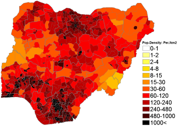
Furthermore, SuperLender, as a whole, is continuing to grow as a digital lending company in Nigeria. It is, however, surprising that SuperLender does not have a significant number of customers in Abuja as well as in the northern Nigerian states, as previously seen in Figure 3(a). These regions contain higher population densities, as may be seen in Figure 9, and may provide SuperLender with opportunity for further growth.
6.2. Future work
Ideally, if further demographics external data were available, arguably the most informative would be the income earnings per customer as this information would better indicate the ability of a customer to repay their loan. Alternatively, since the latitude and longitude positions of each customer are provided, further features may be created by geocoding their position based on regional census data, for example, the average income earned in a region. Additional information, for example, a customer’s income spending ratio, net worth, and number of dependants, would likely also enhance the learning models’ predictive abilities.
During this report, eight supervised learning algorithms were evaluated according to their ability to predict the whether a SuperLender customer would default on their loan. It was found that the CT and RF learning model performed significantly better than the other learning models — a finding which begs the question whether other tree-based/ensemble learning models may also achieve similar or superior performance in this context. Consequently, it may be worthwhile investigating the predictive performance of gradient-boosted decision trees (or XGBoost)