🎓 An Overview of Supervised Machine Learning
Part 1 - Classic Machine Learning Algorithms Series
This blog post was adapted from Sections 4.1, 4.2 and 4.3 in my PhD dissertation.
This is the first post in a series of blog posts where I’ll deep-dive into some of the classic Machine Learning algorithms that have paved the way for the more sophisticated techniques that are changing the world as we know it. In this blog post, I’ll introduce the bread-and-butter machine learning paradigm, Supervised Learning, as well as come practical considerations that come with framing a problem as a supervised learning problem. Let’s get started!
1. Introduction
The term “machine learning” (ML) was first coined by Arthur Samuel in 1954 upon the publication of his self-learning program which could successfully play the game of Checkers
2. Machine learning paradigms
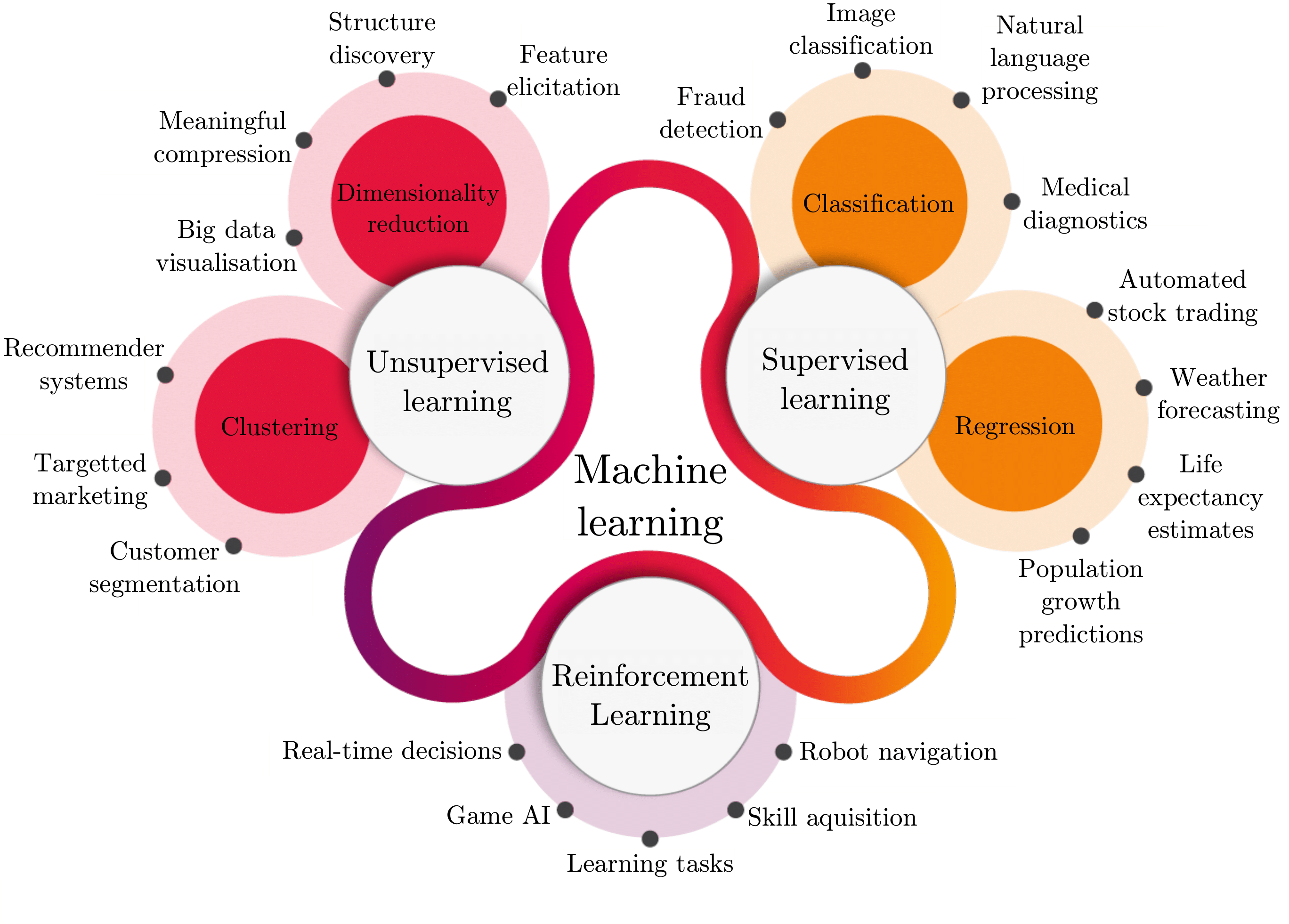
The majority of ML algorithms reside, for the most part, in one of four broad learning paradigms which may be described as follows and is partly illustrated in Figure 1:
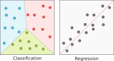
- Supervised learning. In a supervised learning paradigm, an algorithm is presented with a set of labelled data comprising input examples together with known corresponding output values deemed of particular interest. The task of the algorithm is to approximate the underlying function which maps these input examples to their corresponding output values
. In the case where output values are categorical, the problem is called a classification problem while in the case of continuous output values, it is called a regression problem. - Unsupervised learning. In an unsupervised learning paradigm, an algorithm is presented with a set of unlabelled data for which there are no known corresponding output values. The task of the algorithm is to identify some underlying structure (or pattern) between the various input values
. This is typically achieved through dimensionality reduction techniques (which aim to project the data onto a lower dimensional space), density estimation methods (which attempt to construct a functional estimate of the observed data), and/or though the application of various clustering approaches (whereby similar input examples are grouped together). This paradigm is the primary task of exploratory data analysis (EDA) which attempts to first make sense of the acquired data so that meaningful questions can be framed and posed . - Semi-supervised learning. In a semi-supervised learning paradigm, an algorithm is typically presented with both labelled an unlabelled data. In this paradigm, the algorithm utilises both supervised and unsupervised learning techniques to accomplish inductive or transductive learning tasks. In the case of the former, unlabelled data are used in conjunction with a small amount to labelled data to improve the accuracy of a supervised learning task
. In the case of the latter, the aim is to infer the correct labels for each of the unlabelled examples as a way of avoiding the costly and time-consuming task of manual labelling. - Reinforcement learning. Lastly, in a reinforcement learning paradigm, an algorithm, commonly referred to as an agent, is exposed to a dynamic environment which is typically some abstraction of the real world. The task of the agent is to determine, through a trial-and-error process, the correct set of actions (collectively called a policy) which maximises (or minimises) some long-term cumulative reward (or punishment)
. Reinforcement learning differs from supervised learning in that, instead of correcting sub-optimal actions, the focus is on striking a balance between the exploration of uncharted territory and the exploitation of current knowledge .
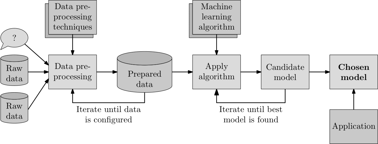
3. The supervised learning procedure
The primary goal of any supervised learning process is to choose an appropriate ML algorithm that can accurately model an underlying relationship between the variables in a data set. The standard process by which this is achieved is illustrated graphically in Figure 2, where the process begins by developing a well-formulated research question. To answer this research question by means of supervised learning, a researcher must first transform one or more sets of raw data (deemed relevant to the current investigation) by means of a host of data preprocessing techniques into a set of prepared data. The process of ensuring that the data are appropriately prepared for the application of an ML algorithm is often iterative in nature, usually requiring the data to be reshaped in such a way that one may draw the best scientific conclusions from them. Once a set of appropriately prepared data has been established, the researcher may apply a selection of supervised ML algorithms to the data in an attempt at predicting a specific feature that is able to provide insight into the original research question. Again, this is an iterative process, whereby the performance of each candidate model is trained and evaluated in respect of the prepared data until an appropriate model has been found. Thereafter, the researcher may draw insight from this model by predicting the outcome of new scenarios presented to the model.
As a way of establishing a set of formal notation and naming conventions for use in the remainder of this blog series, the “input” variables, hereafter referred to as explanatory variables, are denoted by the set $\mathcal{X}={\mathbf{x}^{(1)},\ldots,\mathbf{x}^{(m)}}$ of $m$ vectors, where the $i$th vector of explanatory variables $\mathbf{x}^{(i)}=\langle x_1^{(i)}\cdots x_n^{(i)}\rangle$ has values associated with $n$ explanatory attributes (or features) of interest. All explanatory variables correspond to a set of “output” variables, hereafter referred to as the target variables, which are denoted by $\mathcal{Y}={y^{(1)},\ldots,y^{(m)}}$, where only one target attribute defines this set. A pair of the form $(\mathbf{x}^{(i)}, y^{(i)})$, therefore, denotes the $i$th observation recorded for a specific event, where a vector $\mathbf{x}^{(i)}$ of explanatory variables is mapped to a single target variable $y^{(i)}$. A data set ${(\mathbf{x}^{(1)}, y^{(1)}),\ldots,(\mathbf{x}^{(m)}, y^{(m)})}$ of $m$ independent observations of a specific event is called a sample set. Given such a sample set, the goal of a supervised learning algorithm, hereafter referred to as a learning model, is to learn a function $h:\mathcal{X}\mapsto\mathcal{Y}$ such that, for an unseen vector $\mathbf{x}$, $h(\mathbf{x})=y$ is a “good” predictor of the actual target variable $y$. The function $h(\mathbf{x})$ is called the hypothesis of the learning model and may predict either a categorical or a continuous target variable. Furthermore, if the fundamental working of a learning model is based on a specific assumption of the distribution of observations, it is called a parametric model, while learning models that do not make any explicit assumptions about the distribution of observations are termed non-parametric models.
4. Data taxonomy
Since the primary input to all ML algorithms is data, one must be aware of the many consideration associated with the appropriate understanding, management and manipulation of data in the context of ML. More specifically, one should be able to: (1) Identify the many formats in which attributes in a data set may be expressed, (2) understand the origin of erroneous and missing values in a data set and how they should be corrected appropriately, and (3) be aware of the various data partitioning methods used during the performance evaluation of a learning model.
According to Baltzan and Phillips
The format of data can, in its most primordial form, be classified into two broad categories: Data can either be inherently structured or unstructured. Structured data, for the most part, exhibit a high degree of organisation so that they can be interpreted easily by a computer, while unstructured data do not follow any conventional data structure
The data type of an attribute describes the inherent values a data item can assume and may, in its most basic form, be grouped into one of two categories, namely as a qualitative (categorical) attribute or a quantitative attribute. The latter describes an attribute which is inherently captured on a numerical scale, such as the velocity or mass of an object
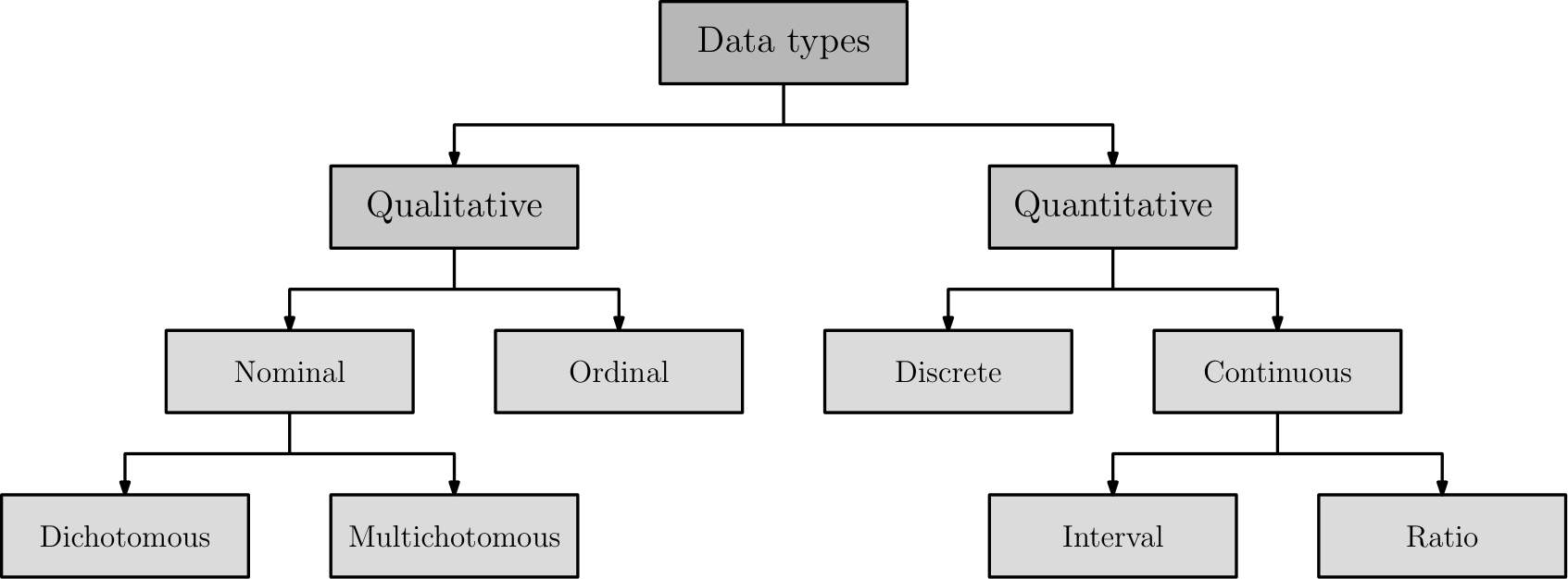
Qualitative attributes may further be categorised into attributes that are either nominal or ordinal in nature
Quantitative attributes may further be categorised into attributes that are either discrete or continuous in nature. Discrete attributes can assume a single value from a finite set of values, such as the number rolled on a six-face die, for example. All qualitative attributes are inherently discrete since they are countable and can assume only a certain set of values. Continuous attributes, on the other hand, can assume one of an uncountably infinite set of values (which exist along a continuum), such as the temperature in a room, for example. Continuous attributes can further be categorised into attributes which assume values on an interval scale or a ratio scale. The latter assumes that there exists a so-called true zero which reflects the absence of the specific measured feature. An object’s weight is, for example, a ratio attribute since a value of zero indicates that the object has no weight. Interval attributes, on the other hand, do not assume this property. Temperature measured in degrees Fahrenheit ($^{\circ}F$) or Celsius ($^{\circ}C$) is, for example, an interval attribute since zero $^{\circ}F$ or $^{\circ}C$ does not imply no temperature. If, however, temperature is measured in Kelvin, then it may be expressed as a ratio estimate, since zero Kelvin indicates the absence of temperature.
5. Data cleaning
Probably the most important and, at the same time, mundane tasks associated with the data preparation process is that of data cleaningAnnual income and Ethnicity have been left blank, the attributes Name, Date of birth and Place of birth are incomplete, and the attribute Sex, although in the correct format, does not reflect the true value.
| Attribute | True data | Actual data |
|---|---|---|
| Name | Maria Margaret Smith | Maria Smith |
| Date of birth | 2/19/1981 | 1981 |
| Sex | F | M |
| Ethnicity | Hispanic and Caucasian | |
| Place of Birth | Nogales, Somora, Mexico | Nogales |
| Annual income | $50,000 |
According to Hellerstein
Since the majority of learning models require a complete data set in order to function properly, it is necessary to address any missing data in a data set. Obviously, the best approach would be to manually fill in all incomplete entries to contain the correct information. This is, however, not always practical, especially if there is a significant proportion of missing values in a considerably large data set. The second approach, which may seem more reasonable, would be to delete any observations with missing values entirely, leaving only the observations that contain values for all of the defined attributes. This may, however, result in a substantial loss in the overall set of observations, to the point where there are too few data to conduct a meaningful investigation. Another approach is to identify those attributes in the data set which possess a large proportion of missing values. If the proportion of missing values of an attribute exceed a specific threshold, then the attribute may be disregarded altogether. The final approach would be to employ a specific imputing technique where missing values are filled according to some specified rule. Many imputing methods have been proposed in the literature, namely: Mean imputation (replace missing values with the average/most frequent value), hot deck imputation (replace missing values with randomly chosen observations of similar values), cold deck imputation (replace missing values with systematically chosen observations of similar values), random imputation (replace missing values with random values) and model-based imputation (construct a learning model to predict missing values based on values of complete observations)
The final activity in the data cleaning process is concerned with the detection of any outliers that may be present in a data set, where an outlier is described as an observation that does not conform to the general pattern observed in a data set
6. Data partitioning methods
The initial sample set is typically partitioned into three separate data sets, namely a training set, a validation set and a testing set

Cross-validation
There are two main types of cross-validation methods, namely: $k$-fold cross-validation and leave-one-out cross-validation. In the case of $k$-fold cross-validation, the set of $m$ observations is partitioned into $k$ equal (or as close to equal as possible) parts (or folds), as illustrated graphically in Figure 5. A total of $k-1$ folds of the data are then used for training a learning model, while the remaining fold is used for model validation. This process is repeated a total of $k$ times, each time using a different fold for validation purposes. The final performance of a learning model is then estimated as the average of the misclassification errors seen during the $k$ repetitions.
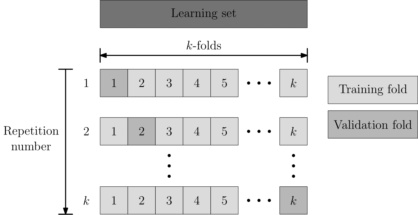
The leave-one-out method of cross-validation is a special case of the $k$-fold cross-validation that occurs when $k=m$ (i.e. $k$ is equal to the number of observations). As its name suggests, all observations, except one (i.e. $m-1$ observations), are used to train the learning model according to this method, and the remaining observation is used for model validation. This procedure is thus repeated a total of $m$ times, where the final performance of a learning model is estimated as the average of the $m$ misclassification errors.
Bootstrap re-sampling
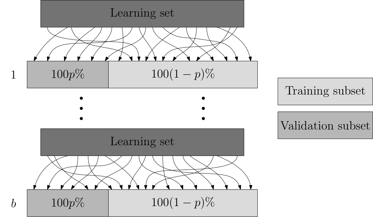
The second type of data sampling method is that of bootstrap re-sampling (or just bootstrapping), where the aim is to create a bootstrap sample of observations for training and validating learning models — the method by which it achieves these subsets is, however, quite different. Bootstrapping involves the repeated selection of observations from the learning set with replacement
7. Performance measures
As previously described in Section 3, the primary goal of any supervised learning procedure is choosing an appropriate model. One must, therefore, be aware of various notions that may assist in selecting, configuring and evaluation a model for a specific learning task. More specifically, one should be able to: (1) Evaluate the performance of a learning model according to an appropriate performance measure, (2) identify whether a learning algorithm is generalising the data, and (3) appreciate the trade-off associated with employing a complex learning model rather than one that is easier to understand. These topics are discussed in the remainder or the blog post.
Since the evaluation of a learning model is essential in any ML investigation, one must be able to choose a performance measure that is most appropriate when presented with either a classification or regression task. In the case of the latter, the most popular performance measures are the well-known mean square error, mean absolute error and R-squared error

Perhaps the best-known performance measure is classification accuracy (CA), which describes the total proportion of correct predictions made by a learning model, expressed mathematically as
\begin{equation} \text{CA}=\frac{\text{TP}+\mbox{TN}}{\text{TP}+\text{FP}+\text{FN}+\text{TN}}. \end{equation}
Although CA seems to be an intuitive measure by which to assess a classifier, it should never be used when there is a large category imbalance in a data set. Consider, for example, a case in which $950$ positive observations and $50$ negative observations are contained in a data set. Then a learning model can easily achieve a CA of $95\%$ simply by always predicting the majority category (i.e. the positive category).
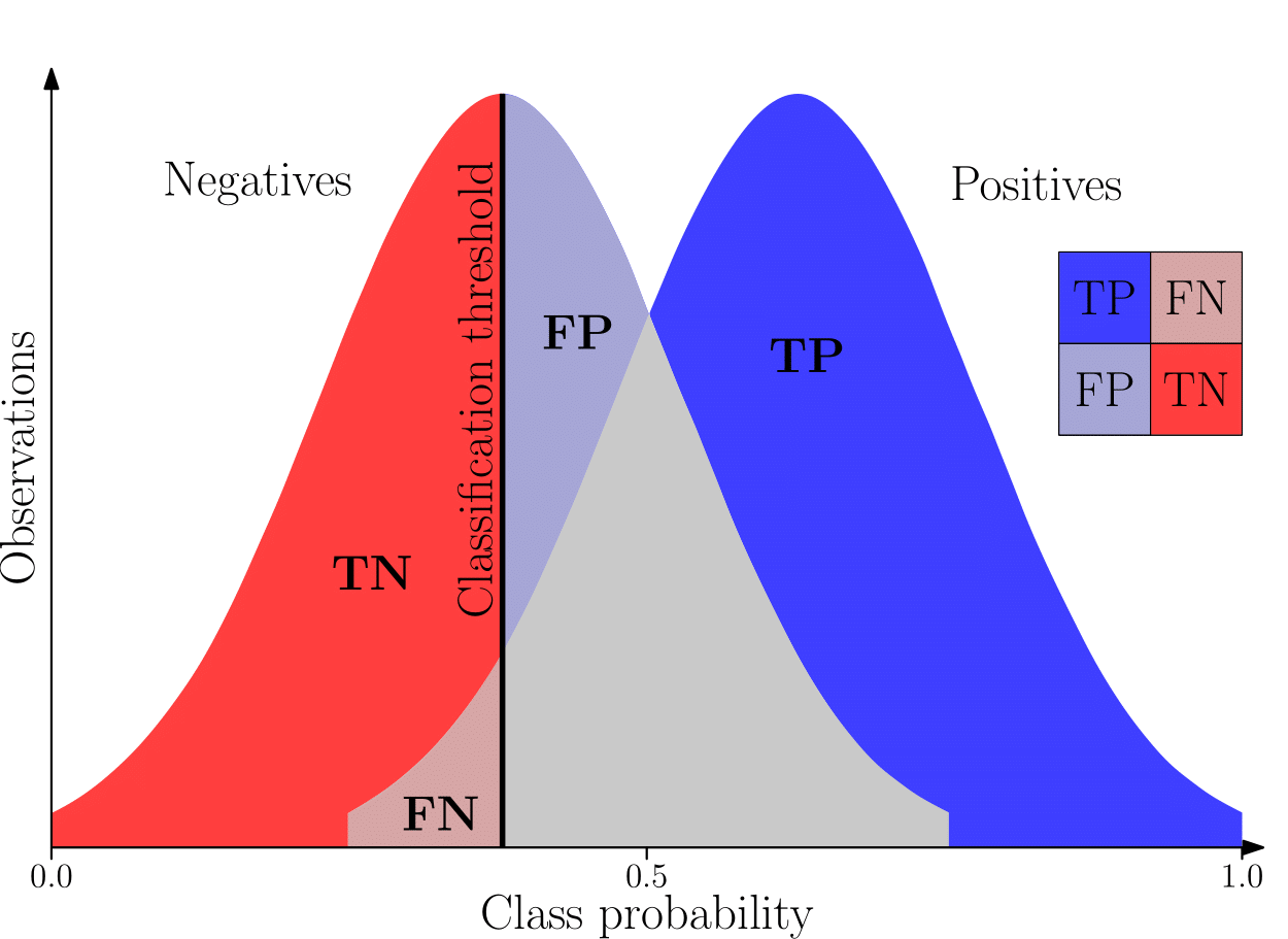
In order to overcome this flaw, the performance of a learning model can instead be described in terms of two separate measures, namely precision and recall. Precision describes what proportion of the observations predicated as positive are actually positive observations, expressed mathematically as
\begin{equation} \mbox{Precision}=\frac{\mbox{TP}}{\mbox{TP}+\mbox{FP}}.\label{4.eqn.precision} \end{equation}
Recall (also known as sensitivity) describes what proportion of the observations that are actually positive were correctly classified as positive, expressed mathematically as
\begin{equation} \mbox{Recall}=\frac{\mbox{TP}}{\mbox{TP}+\mbox{FN}}.\label{4.eqn.recall} \end{equation}
Although these two performance measures can be used together to measure the performance of a single learning model, in the case when two learning models are compared, it is not always clear which learning model achieves superior performance. For this reason, an alternative performance measure, called the $\text{F}_{\beta}$-score is defined as
\begin{equation} \text{F}_{\beta}=\left(\frac{1}{\beta\left(\frac{1}{\text{Precision}}\right)+(1-\beta)\left(\frac{1}{\text{Recall}}\right)}\right).\label{4.eqn.fbeta} \end{equation}
This score is a weighted harmonic mean of precision and recall in which $\beta$ is a weight parameter used to specify the importance of precision over recall. The choice of $\beta$ is, to a large extent, problem-specific. A value of $\beta$ close to one essentially reduces (\ref{4.eqn.fbeta}) to (\ref{4.eqn.precision}), while a value of $\beta$ close to zero reduces (\ref{4.eqn.fbeta}) to (\ref{4.eqn.recall}). A $\beta$-value of $b=0.5$ weights both precision and recall equally and is known in statistics as the F$_1$-score.
Arguably the most popular classification performance measure is the area under curve (AUC) performance measure
\begin{equation} \text{TPR}=\frac{\text{TP}}{\text{TP}+\text{FN}}=\text{Recall}, \end{equation}
while its FPR may be expressed as
\begin{equation} \text{FPR}=\frac{\text{FP}}{\text{FP}+\text{TN}}. \end{equation}
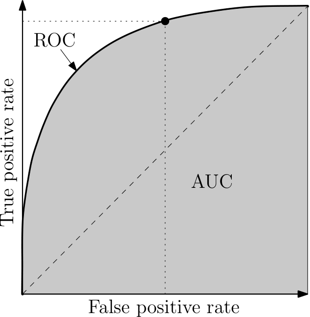
The area under the ROC curve (or just the AUC) indicates to what extent a model is able to distinguish between positive and negative observations. The AUC score may also be interpreted as the probability that a learning model ranks a randomly chosen positive observation higher than a random negative observation. An AUC score of one is, therefore, the most ideal scenario as it indicates that a learning model can perfectly distinguish between positive and negative categories. An AUC score of zero indicates that the learning model is, in fact, reciprocating the categories (i.e. positive observations are always predicted as negative and vice versa). In actuality, this is also an ideal scenario since merely inverting the predictions of the learning model would produce a perfect classifier. An AUC score of $0.5$ (indicated by the area under the dashed line in Figure 7(b)), on the other hand, is the worst-case scenario as it indicates that a learning model has no discrimination capacity to distinguish between the positive and negative categories (i.e. the learning model is no better than random guessing)
8. Overfitting vs underfitting the training data
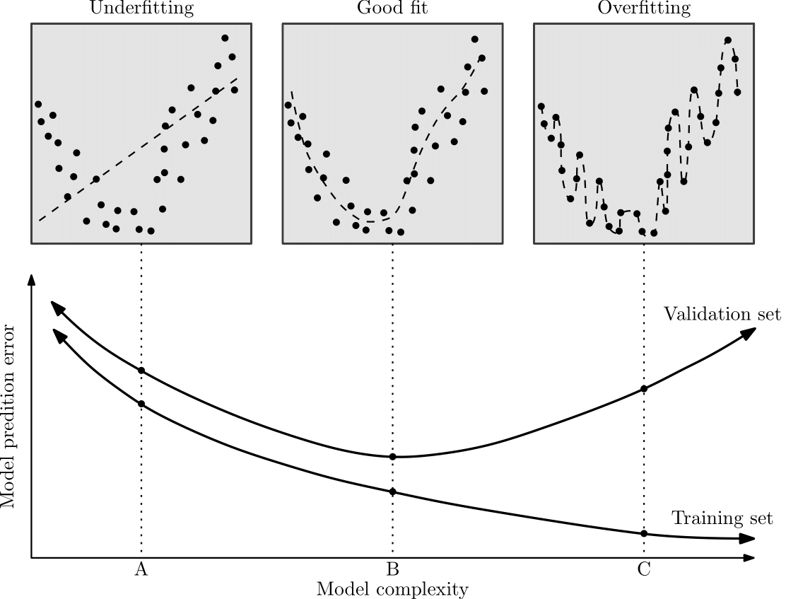
One of the most fundamental concepts to grasp in ML is the notion of a learning model underfitting or overfitting a set of training data. Underfitting occurs when a learning model does not perform well in respect of either the training set or the validation set, as illustrated by a learning model with a complexity of “A” in Figure 8. In this case, the model is too simple and cannot model the underlying pattern (or trend) in the training set, resulting in a poor ability to predict unseen observations accurately. Overfitting, on the other hand, occurs when a learning model performs well in respect of the training set, but significantly poor in respect of the validation set, as illustrated by a learning model with a complexity of “C” in Figure 8. In this case, the learning model is not learning the underlying trend. It is rather memorising the observations in the training set, again resulting in a poor generalisation ability (and thus a poor prediction performance) in respect of unseen observations. An ideal learning model is, therefore, one that achieves a suitable trade-off between underfitting and overfitting the observations in the training set, as illustrated by a learning model with a complexity of “B” in Figure 8. In this case, the learning model is able to generalise the underlying trend displayed appropriately by the observations in the training set which result in a better overall prediction performance in respect of unseen observations.
9. Model performance vs model interpretability
Understanding why an ML model makes a specific prediction may, in many applications, be just as crucial as the accuracy of the prediction itself. A model that is interpretable creates a certain degree of trust in its predictions, provides insights into the process being modelled, and highlights potential biases present in the data under consideration. The lack of interpretability of many ML models (often called black-box models) is a frequent barrier to their adoption, since end-users typically prefer solutions that are understandable to a human
The ethical considerations associated with autonomous vehicles, for example, are often called into question since the learning models (typically reinforcement learning algorithms
10. Wrapping up
And that’s it! In this blog post, I walked you through arguably the most well-known machine learning paradigm, supervised learning, as well as some considerations you probably want to bear in mind when framing a problem as a supervised learning problem. Join me in my next blog post where I’ll go deep into a whole branch of statistical learning models, namely Generalised Linear Models (GLMs). See you there!